Digit Detector: Building Your First AI Model to Recognize Handwritten Digits
A Complete Beginner’s Guide to Creating, Training, and Deploying a Digit Classification Model
Introduction
Have you ever wondered how computers can recognize handwritten digits? In this comprehensive tutorial, we’ll build an AI model from scratch that can identify and classify handwritten digits (0-9) with impressive accuracy.

What We’ll Build
We’re creating a Convolutional Neural Network (CNN) that can:
- Take an image of a handwritten digit as input
- Process and analyze the image
- Output a prediction of which digit (0-9) it represents
- Achieve over 95% accuracy on test data
Why Use the MNIST Dataset?
The MNIST dataset is the perfect starting point for beginners because:
What is MNIST?
- Modified National Institute of Standards and Technology database
- Contains 70,000 images of handwritten digits (0-9)
- Each image is 28x28 pixels in grayscale
- Already split into training (60,000) and testing (10,000) sets
Why MNIST is Ideal for Learning:
- Small and manageable: Quick to download and train
- Well-preprocessed: Images are already cleaned and normalized
- Benchmark dataset: You can compare your results with others
- Perfect complexity: Not too simple, not too complex for beginners
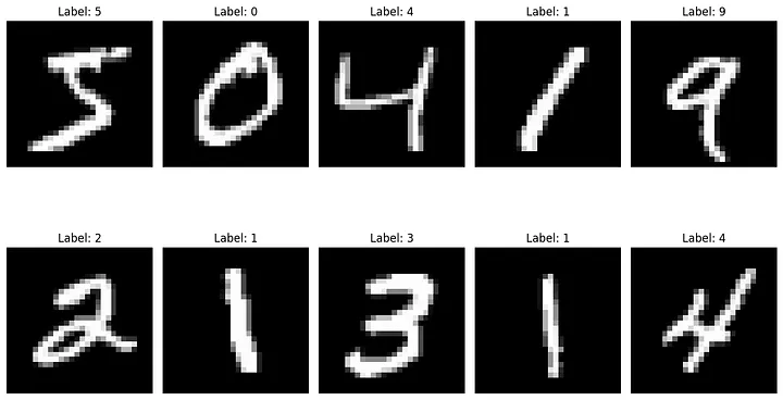 Sample images from the MNIST dataset showing various handwritten digits
Prerequisites and Setup
Before we start coding, let’s understand what we need and why:
Required Libraries
1
2
3
4
5
6
# Core libraries for our project
import tensorflow as tf          # Deep learning framework
import numpy as np              # Numerical computing
import matplotlib.pyplot as plt # Data visualization
from sklearn.metrics import classification_report, confusion_matrix
import seaborn as sns          # Enhanced visualization
Why these libraries?
- TensorFlow: Google’s deep learning framework - handles neural network creation and training
- NumPy: Essential for array operations and mathematical computations
- Matplotlib: Creates plots to visualize our data and results
- Scikit-learn: Provides evaluation metrics to assess model performance
- Seaborn: Makes beautiful statistical visualizations
Installation
1
pip install tensorflow numpy matplotlib scikit-learn seaborn
Step 1: Loading and Exploring the Data
Let’s start by loading our dataset and understanding what we’re working with:
1
2
3
4
5
6
7
8
9
10
11
12
# Load the MNIST dataset
(x_train, y_train), (x_test, y_test) = tf.keras.datasets.mnist.load_data()

# Let's explore our data
print("Training data shape:", x_train.shape)
print("Training labels shape:", y_train.shape)
print("Test data shape:", x_test.shape)
print("Test labels shape:", y_test.shape)

# Check the range of pixel values
print("Pixel value range:", x_train.min(), "to", x_train.max())
print("Number of classes:", len(np.unique(y_train)))
What’s happening here?
tf.keras.datasets.mnist.load_data()downloads and loads the MNIST dataset- We get training data (x_train, y_train) and test data (x_test, y_test)
- x_train/x_test: Images (features)
- y_train/y_test: Labels (what digit each image represents)
 Visual representation of our data structure
Visualizing Sample Images
1
2
3
4
5
6
7
8
9
10
11
12
13
# Function to display sample images
def plot_sample_images(images, labels, num_samples=10):
    plt.figure(figsize=(12, 8))
    for i in range(num_samples):
        plt.subplot(2, 5, i + 1)
        plt.imshow(images[i], cmap='gray')
        plt.title(f'Label: {labels[i]}')
        plt.axis('off')
    plt.tight_layout()
    plt.show()

# Display sample training images
plot_sample_images(x_train, y_train)
Why visualize the data?
- Helps us understand what our model will be learning from
- Identifies potential issues (blurry images, incorrect labels)
- Gives us intuition about the task difficulty
Sample handwritten digits from our training dataset
Step 2: Data Preprocessing
Raw data is rarely ready for machine learning. Let’s prepare our data:
Normalization
1
2
3
4
5
6
# Normalize pixel values to be between 0 and 1
x_train = x_train.astype('float32') / 255.0
x_test = x_test.astype('float32') / 255.0

print("After normalization:")
print("Training data range:", x_train.min(), "to", x_train.max())
Why normalize?
- Original range: Pixel values are 0-255 (integers)
- After normalization: Values become 0-1 (floats)
- Benefits:
- Faster training (smaller numbers are easier to compute)
- Better convergence (prevents certain features from dominating)
- Numerical stability
Reshaping for CNN
1
2
3
4
5
6
7
# Reshape data to add channel dimension for CNN
x_train = x_train.reshape(x_train.shape[0], 28, 28, 1)
x_test = x_test.reshape(x_test.shape[0], 28, 28, 1)

print("Reshaped data:")
print("Training shape:", x_train.shape)
print("Test shape:", x_test.shape)
Why reshape?
- CNNs expect input in format: (batch_size, height, width, channels)
- Our images are grayscale (1 channel) vs RGB (3 channels)
- The “1” at the end indicates 1 color channel
One-Hot Encoding Labels
1
2
3
4
5
6
7
8
9
# Convert labels to one-hot encoding
y_train_categorical = tf.keras.utils.to_categorical(y_train, 10)
y_test_categorical = tf.keras.utils.to_categorical(y_test, 10)

print("Original label shape:", y_train.shape)
print("One-hot encoded shape:", y_train_categorical.shape)
print("\nExample transformation:")
print("Original label:", y_train[0])
print("One-hot encoded:", y_train_categorical[0])
What is One-Hot Encoding?
- Converts categorical labels to binary vectors
- Example: digit “3” becomes [0, 0, 0, 1, 0, 0, 0, 0, 0, 0]
- Why needed: Neural networks work better with this format for classification
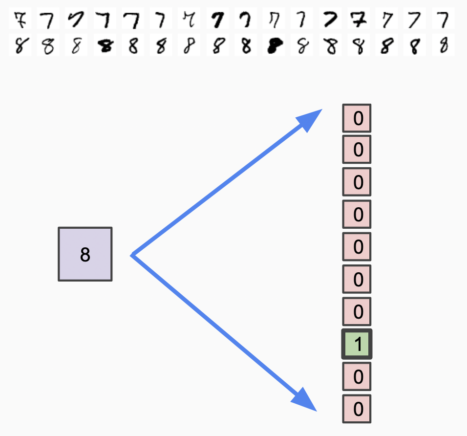
Visual explanation of one-hot encoding transformation
Step 3: Building the CNN Model
Now for the exciting part - creating our neural network!
Understanding CNN Architecture
1
2
3
4
5
6
7
8
9
10
11
12
13
14
15
16
17
18
19
20
21
22
23
24
25
26
27
def create_cnn_model():
    model = tf.keras.Sequential([
        # First Convolutional Block
        tf.keras.layers.Conv2D(32, (3, 3), activation='relu', input_shape=(28, 28, 1)),
        tf.keras.layers.MaxPooling2D((2, 2)),

        # Second Convolutional Block
        tf.keras.layers.Conv2D(64, (3, 3), activation='relu'),
        tf.keras.layers.MaxPooling2D((2, 2)),

        # Third Convolutional Block
        tf.keras.layers.Conv2D(64, (3, 3), activation='relu'),

        # Flatten and Dense Layers
        tf.keras.layers.Flatten(),
        tf.keras.layers.Dense(64, activation='relu'),
        tf.keras.layers.Dropout(0.5),
        tf.keras.layers.Dense(10, activation='softmax')
    ])

    return model

# Create the model
model = create_cnn_model()

# Display model architecture
model.summary()
Let’s break down each layer:
- Conv2D(32, (3, 3)):
- Creates 32 feature maps using 3x3 filters
- Detects edges, patterns, and basic features
- Why 32? Good balance between complexity and computational efficiency
- MaxPooling2D(2, 2):
- Reduces image size by taking maximum value in 2x2 windows
- Purpose: Reduces computational load and prevents overfitting
- Makes the model focus on the most important features
- Progressive Filter Increase (32 → 64 → 64):
- Deeper layers detect more complex patterns
- First layer: edges and basic shapes
- Later layers: digit-specific patterns
- Flatten():
- Converts 2D feature maps to 1D vector
- Why: Dense layers expect 1D input
- Dense(64):
- Fully connected layer that combines all features
- ReLU activation: Allows non-linear learning
- Dropout(0.5):
- Randomly “turns off” 50% of neurons during training
- Purpose: Prevents overfitting
- Dense(10, softmax):
- Output layer with 10 neurons (one per digit)
- Softmax: Converts outputs to probabilities that sum to 1
 Visual representation of our CNN architecture
Compiling the Model
1
2
3
4
5
6
# Compile the model
model.compile(
    optimizer='adam',
    loss='categorical_crossentropy',
    metrics=['accuracy']
)
Explanation of compilation parameters:
- Adam optimizer: Adaptive learning rate algorithm (usually works well)
- Categorical crossentropy: Loss function for multi-class classification
- Accuracy metric: Easy to understand performance measure
Step 4: Training the Model
Time to teach our model to recognize digits!
Setting Up Training
1
2
3
4
5
6
7
8
9
10
11
12
13
14
15
16
17
18
19
20
21
22
23
# Define callbacks for better training
early_stopping = tf.keras.callbacks.EarlyStopping(
    monitor='val_loss',
    patience=3,
    restore_best_weights=True
)

reduce_lr = tf.keras.callbacks.ReduceLROnPlateau(
    monitor='val_loss',
    factor=0.2,
    patience=2,
    min_lr=0.0001
)

# Train the model
history = model.fit(
    x_train, y_train_categorical,
    batch_size=128,
    epochs=20,
    validation_data=(x_test, y_test_categorical),
    callbacks=[early_stopping, reduce_lr],
    verbose=1
)
What are callbacks and why use them?
- EarlyStopping: Stops training if model stops improving
- Prevents wasting time and overfitting
patience=3: Wait 3 epochs before stopping
- ReduceLROnPlateau: Reduces learning rate when stuck
- Helps fine-tune the model when improvement slows
factor=0.2: Multiply learning rate by 0.2
Training parameters explained:
- batch_size=128: Process 128 images at once (memory vs speed trade-off)
- epochs=20: Maximum training cycles through entire dataset
- validation_data: Use test set to monitor overfitting
Visualizing Training Progress
1
2
3
4
5
6
7
8
9
10
11
12
13
14
15
16
17
18
19
20
21
22
23
24
# Plot training history
def plot_training_history(history):
    fig, (ax1, ax2) = plt.subplots(1, 2, figsize=(12, 4))

    # Plot accuracy
    ax1.plot(history.history['accuracy'], label='Training Accuracy')
    ax1.plot(history.history['val_accuracy'], label='Validation Accuracy')
    ax1.set_title('Model Accuracy')
    ax1.set_xlabel('Epoch')
    ax1.set_ylabel('Accuracy')
    ax1.legend()

    # Plot loss
    ax2.plot(history.history['loss'], label='Training Loss')
    ax2.plot(history.history['val_loss'], label='Validation Loss')
    ax2.set_title('Model Loss')
    ax2.set_xlabel('Epoch')
    ax2.set_ylabel('Loss')
    ax2.legend()

    plt.tight_layout()
    plt.show()

plot_training_history(history)

Training and validation accuracy/loss over epochs
Step 5: Evaluating the Model
Let’s see how well our model performs:
Basic Evaluation
1
2
3
4
5
6
7
8
# Evaluate on test set
test_loss, test_accuracy = model.evaluate(x_test, y_test_categorical, verbose=0)
print(f"Test Accuracy: {test_accuracy:.4f}")
print(f"Test Loss: {test_loss:.4f}")

# Make predictions
predictions = model.predict(x_test)
predicted_classes = np.argmax(predictions, axis=1)
Detailed Analysis with Confusion Matrix
1
2
3
4
5
6
7
8
9
10
11
12
13
14
15
# Create confusion matrix
cm = confusion_matrix(y_test, predicted_classes)

# Plot confusion matrix
plt.figure(figsize=(10, 8))
sns.heatmap(cm, annot=True, fmt='d', cmap='Blues',
            xticklabels=range(10), yticklabels=range(10))
plt.title('Confusion Matrix')
plt.xlabel('Predicted Label')
plt.ylabel('True Label')
plt.show()

# Print classification report
print("\nClassification Report:")
print(classification_report(y_test, predicted_classes))
Understanding the Confusion Matrix:
- Rows: True labels
- Columns: Predicted labels
- Diagonal: Correct predictions
- Off-diagonal: Misclassifications
 Confusion matrix showing model performance per digit
Analyzing Misclassifications
1
2
3
4
5
6
7
8
9
10
11
12
13
14
15
# Find misclassified examples
misclassified_indices = np.where(predicted_classes != y_test)[0]

# Display some misclassified images
def show_misclassified(indices, num_examples=8):
    plt.figure(figsize=(12, 8))
    for i, idx in enumerate(indices[:num_examples]):
        plt.subplot(2, 4, i + 1)
        plt.imshow(x_test[idx].reshape(28, 28), cmap='gray')
        plt.title(f'True: {y_test[idx]}, Pred: {predicted_classes[idx]}')
        plt.axis('off')
    plt.tight_layout()
    plt.show()

show_misclassified(misclassified_indices)
 Examples of digits our model got wrong - helps us understand limitations
Step 6: Saving the Model
Now let’s save our trained model for future use:
Saving in TensorFlow Format
1
2
3
4
5
6
7
# Save the entire model
model.save('digit_detector_model.h5')
print("Model saved as 'digit_detector_model.h5'")

# Alternative: Save in TensorFlow SavedModel format
model.save('digit_detector_savedmodel')
print("Model saved as 'digit_detector_savedmodel'")
Loading the Model
1
2
3
4
5
6
7
# Load the saved model
loaded_model = tf.keras.models.load_model('digit_detector_model.h5')
print("Model loaded successfully!")

# Verify it works
test_prediction = loaded_model.predict(x_test[:5])
print("Test predictions:", np.argmax(test_prediction, axis=1))
Why save models?
- Avoid retraining every time
- Share with others
- Deploy to production
- Continue training later
Creating a Prediction Function
1
2
3
4
5
6
7
8
9
10
11
12
13
14
15
16
17
18
19
20
21
def predict_digit(model, image):
    """
    Predict digit from a single image
    """
    # Ensure image is in correct format
    if image.shape != (28, 28, 1):
        image = image.reshape(1, 28, 28, 1)
    else:
        image = image.reshape(1, 28, 28, 1)

    # Make prediction
    prediction = model.predict(image, verbose=0)
    predicted_digit = np.argmax(prediction)
    confidence = np.max(prediction)

    return predicted_digit, confidence

# Test the function
sample_image = x_test[0]
digit, confidence = predict_digit(model, sample_image)
print(f"Predicted digit: {digit}, Confidence: {confidence:.4f}")